Fast Multipole Acceleration#
FMM accelerates the Green’s function interactions for problems of the structrue
Without compression this is dense interaction work: storage is roughly \(O(MN)\) and a direct matrix vector product is also \(O(MN)\).
The fast multipole method avoids treating all interactions equally. Nearby interactions are kept accurate and direct while far interactions are approximated by expansions around cluster centers.
Where FMM Enters BEM#
A Galerkin BEM matrix is built from a double boundary integral. For a scalar single layer operator the discrete matrix entries are
After quadrature, the kernel interaction part of this matrix vector product becomes a source target operation: source contributions are formed from the trial density, the kernel \(G(x,y)\) is evaluated between source and target quadrature points, and the target values are accumulated back into the test space.
In the NGSolve BEM implementation, the final operator is not only the FMM approximation. It is assembled as
where \(A_{\mathrm{corr}}\) is a sparse near field correction. It replaces unreliable close interactions by accurate local integration, including Sauter Schwab [SS09] rules for singular and nearly singular boundary element pairs.
Near Field and Far Field#
For a target cluster, source interactions are split into two classes:
near field: source and target clusters are close - these terms are evaluated directly or corrected by special quadrature,
far field: clusters are well separated - their combined effect is represented by multipole and local expansions.
For Helmholtz type kernels, the far field expansion uses spherical harmonics together with spherical Bessel and Hankel functions. Many source points are summarized by a small set of expansion coefficients; the expansion is then evaluated for many target points.
Regular and Singular Expansions#
Following [GD04], the Helmholtz basis functions in spherical coordinates:
Here \(r=|x-c|\), \(Y_n^m\) are spherical harmonics, \(j_n\) are spherical Bessel functions, and \(h_n^{(1)} = j_n + i y_n\) are outgoing spherical Hankel functions.
Regular expansion:
finite at the expansion center,
used for local target expansions.
Singular expansion:
singular at the expansion center,
outgoing for Helmholtz; satisfies the Sommerfeld radiation condition,
used to represent the field generated by a source cluster.
Bessel and Hankel Stability#
The radial basis functions satisfy the recurrence
Numerical issues:
\(j_n(z)\) and \(y_n(z)\) have very different magnitudes for small \(|z|\) and large \(n\),
\(y_n(z)\) is singular at \(z=0\),
\(h_n^{(1)}(z)=j_n(z)+i y_n(z)\) inherits the singular behavior,
direct recurrence can overflow, underflow,
translation coefficients can amplify badly balanced radial factors.
NGSolve avoids evaluating these functions as naive high order closed forms. The regular part is computed by a stable backward recurrence, with special treatment for small arguments. Large intermediate values are renormalized internally so that the recurrence stays in a numerically useful range. The same normalization idea is used when coefficients are translated between regular and singular expansions, so the two representations remain balanced during the FMM passes.
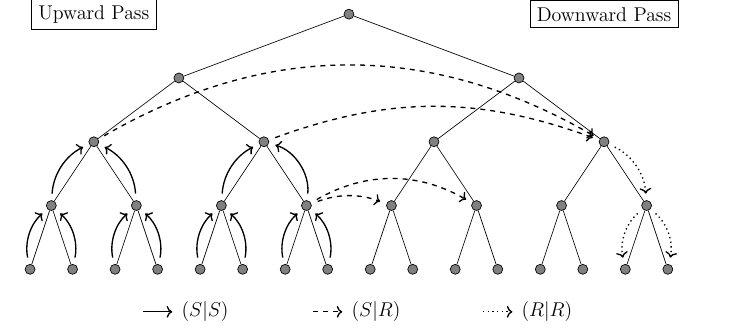
Multilevel FMM#
The implementation uses an adaptive tree structure instead of a single global partition. Source and target points are grouped into boxes. The algorithm then consists of two main passes:
upward pass: leaf boxes collect source contributions into singular multipole expansions; child expansions are translated to parent boxes,
interaction step: well separated singular source expansions are converted into regular local expansions for target boxes,
downward pass: parent regular local expansions are propagated to child target boxes.
Translation types:
FMM Controls#
FMM can be enabled or disabled per boundary integral operator.
A_fmm = LaplaceSL(u * ds, use_fmm=True) * v * ds
A_direct = LaplaceSL(u * ds, use_fmm=False) * v * ds
FMM parameters are exposed as keyword arguments:
A = HelmholtzSL(
    u * ds,
    kappa,
    fmm_maxdirect=100,
    fmm_minorder=20,
    fmm_order_factor=2.0,
    fmm_separation=2.0,
    fmm_eval_separation=3.0,
) * v * ds
GetFMMInfo() returns tree and operator data for the generated FMM matrix action.
info = A_fmm.GetFMMInfo()

info["kernel_name"]
info["source_size"], info["target_size"]
info["nearfield_fraction"]
info["multipole_memory_mb"]
info["source"]["depth"], info["target"]["depth"]
info["source"]["order_min"], info["source"]["order_max"]