Maxwell Stabilized#
We consider a perfect conductor \(\Omega \subset \mathbb R^3\) emitting an electric field into \(\Omega^c\). The scattered electric field \(\boldsymbol E\) solves the following Dirichlet boundary value problem:
The electric field \(\boldsymbol E\) is given by
The classical variational formulation is: find \(j\in H^{-\frac12}(\mathrm{div}_\Gamma,\Gamma)\) such that for all \(\phi\in H^{-\frac12}(\mathrm{div}_\Gamma,\Gamma)\)
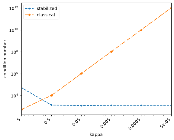
It is well known that the numerical schemes which rely on the classical second order equation are not stable when passing to the limit \(\kappa \to 0\), with condition number \(\mathcal O (\kappa^{-2})\) [Weg11]. The reason for this is that the Gaussian law, which is implicitly embedded for normal wave numbers, is no longer satisfied.
The stabilized system
is conditioned with \(\mathcal O(1)\). We solve the discretized system
where \(\phi_k, \phi_l \in H^{-\frac12}(\mathrm{div}_\Gamma, \Gamma)\) and \(\nu_l, \nu_k\in H^{-\frac12}(\Gamma)\)
We achieve a stabilization for the low frequency range at the cost of a larger system of equations. It is important to note that the stabilized system has a one dimensional kernel that must be explicitly considered.
import netgen.meshing as meshing
import numpy as np
from netgen.occ import *
from ngsolve.la import EigenValues_Preconditioner
from ngsolve import *
from ngsolve.bem import *
from ngsolve.webgui import Draw
from ngsolve.krylovspace import GMRes
import matplotlib.pyplot as plt
def compute_condition_number(mat):
    """Compute condition number via SVD."""
    s = np.linalg.svd(mat.ToDense(), compute_uv=False)
    s_nonzero = s[s > 1e-14 * s[0]]
    return (s_nonzero[0] / s_nonzero[-2], s) # exclude the one dimensional kernel
def solve_stabilized(mesh, kappa, order=1, intorder=4, use_fmm=True):
    fes_hdiv = HDivSurface(mesh, order=order, complex=True)
    fes_l2 = SurfaceL2(mesh, order=order-1, complex=True, dual_mapping=True)
    fes = fes_hdiv * fes_l2
    (uHDiv, uL2), (vHDiv, vL2) = fes.TnT()
    E_inc = CF((1, 0, 0)) * exp(-1j * kappa * z)
    dsi = ds(bonus_intorder=intorder)

    with TaskManager():
        A_kappa = HelmholtzSL( uHDiv.Trace()*dsi , kappa, use_fmm=use_fmm) * vHDiv.Trace() * dsi
        V_kappa = HelmholtzSL( uL2 * dsi , kappa, use_fmm=use_fmm) * vL2 * dsi
        Q_kappa = HelmholtzSL( div(uHDiv.Trace())*dsi , kappa, use_fmm=use_fmm) * vL2 * dsi

        rhs = LinearForm(E_inc * vHDiv.Trace() * dsi).Assemble()
        lhs = A_kappa.mat + Q_kappa.mat + Q_kappa.mat.T + kappa * kappa * V_kappa.mat
        preBlock = BilinearForm( uHDiv.Trace() * vHDiv.Trace() * ds + uL2 * vL2 * ds).Assemble().mat.Inverse(freedofs=fes.FreeDofs())
        sol = GMRes(A=lhs, b=rhs.vec, pre=preBlock, maxsteps=3000, tol=1e-8, printrates=False)

    return lhs, sol, fes, None
def solve_classical(mesh, kappa, order=1, intorder=4, use_fmm=True):
    fes = HDivSurface(mesh, order=order, complex=True)
    u, v = fes.TnT()
    E_inc = CF((1, 0, 0)) * exp(-1j * kappa * z)
    rhs = LinearForm(E_inc * v.Trace() * ds(bonus_intorder=10)).Assemble()
    j = GridFunction(fes)
    dsi = ds(bonus_intorder=intorder)

    with TaskManager():
        V1 = HelmholtzSL( u.Trace()*dsi , kappa, use_fmm=use_fmm) * v.Trace() * dsi
        V2 = HelmholtzSL( div(u.Trace()) * dsi, kappa, use_fmm=use_fmm) * div(v.Trace()) * dsi
        V = V1.mat - 1/(kappa**2) * V2.mat
        pre = BilinearForm(u.Trace() * v.Trace() * ds).Assemble().mat.Inverse(freedofs=fes.FreeDofs())
        success = GMRes(A=V, pre=pre, b=rhs.vec, x=j.vec, tol=1e-10, maxsteps=500, printrates=False)

    return V, j, fes, success
def test_low_frequency_stability():
    radius = 1
    sp = Sphere((0, 0, 0), radius)
    mesh = Mesh(OCCGeometry(sp).GenerateMesh(maxh=1, perfstepsend=meshing.MeshingStep.MESHSURFACE)).Curve(4)

    order = 1
    intorder = 4
    use_fmm=False

    kappa_values = [5.0, 0.5, 0.05, 0.005, 0.0005, 0.00005]
    results_stabilized = []
    results_classical = []

    for kappa in kappa_values:
        try:
            A_mat, sol, fes, _ = solve_stabilized(mesh, kappa, order, intorder, use_fmm)
            cond, lams = compute_condition_number(A_mat)
            results_stabilized.append((kappa, A_mat, sol, fes, cond, mesh, cond, lams))

            A_mat, j, fes, success = solve_classical(mesh, kappa, order, intorder, use_fmm)
            cond, lams = compute_condition_number(A_mat)
            results_classical.append((kappa, A_mat, j, fes, mesh, success, cond, lams))

        except Exception as e:
            print("{:10.4f} | Error: {}".format(kappa, e))

    return results_stabilized, results_classical
results_stabilized, results_classical = test_low_frequency_stability()
Comparison of the eigenvalue distribution#
def plot_lams(lams_stab, lams_class, title):
    plt.plot(lams_stab, label="stabilized", marker=".")
    plt.plot(lams_class, label="classical", marker="*")
    plt.yscale("log")
    plt.legend()
    plt.xlabel("ndof")
    plt.ylabel("lams")
    plt.title(title)
    plt.show()

prev_cond_stab = None
prev_cond_class = None
show_plots = False

if show_plots:
    for i, ((k_stab, *_, cond_stab, lams_stab), (k_class, *_, cond_class, lams_class)) in enumerate(zip(results_stabilized, results_classical)):
        print(f"kappa: {k_stab}")
        if i == 0:
            print(f"stabilized: cond = {round(cond_stab,3)}")
            print(f"classical: cond = {round(cond_class,3)}")

        if prev_cond_stab is not None:
            print(f"stabilized: ratio = {round(cond_stab/prev_cond_stab,3)}, cond = {round(cond_stab,3)}, prev_cond = {round(prev_cond_stab,3)}")
            print(f"classical: ratio = {round(cond_class/prev_cond_class,3)}, cond = {round(cond_class,3)}, prev_cond = {round(prev_cond_class,3)}")

        plot_lams(lams_stab, lams_class, title=f"kappa={k_stab}")

        prev_cond_stab = cond_stab
        prev_cond_class = cond_class
We notice that the condition number of the classical solution grows with \(O(\kappa^{-2})\) whilst the condition number of the stabilized formulation stays constant.
Stability of system matrices#
kappas_stabilized = []
condition_numbers_stabilized = []
kappas_classical = []
condition_numbers_classical = []
for (rs, rc) in zip(results_stabilized, results_classical):
    kappas_stabilized.append(rs[0])
    condition_numbers_stabilized.append(rs[6])
    kappas_classical.append(rc[0])
    condition_numbers_classical.append(rc[6])
plt.xlim(max(kappas_stabilized), min(kappas_stabilized))
plt.loglog(kappas_stabilized, condition_numbers_stabilized, "--", marker=".", label="stabilized")
plt.loglog(kappas_classical, condition_numbers_classical, "-.", marker="*", label="classical")
xs = np.unique(np.r_[kappas_stabilized, kappas_classical])
plt.xticks(xs, [f"{x:g}" for x in xs], rotation=45, ha="right")
plt.legend()
plt.xlabel("kappa")
plt.ylabel("condition number")
plt.show()
References (theoretical and numerical results):