Nearfield Potential Evaluation

After computing the density on the surface, the potential

\[\begin{align*} u(x)=\int_{\Gamma}G(x,y)\,\rho(y)\,dy, \qquad x \in \Omega \setminus \Gamma, \end{align*}\]

away from or close to the boundary needs to be evaluated.

For target points close to the surface, the kernel is nearly singular. Fixed order quadrature and pure farfield expansions lose accuracy exactly where the visualized potential is often most interesting.

Local Geometry

For a close triangular source element \(\phi(\widehat T)\), we project the target point onto the reference triangle and build a tangent triangle at the projected point:

\[ \widehat x_0=\operatorname*{arg\,min}_{\widehat x\in\widehat T}|x-\phi(\widehat x)|, \qquad x_0=\phi(\widehat x_0), \qquad \phi_{\mathrm{lin}}(\widehat x) =\phi(\widehat x_0)+\phi'(\widehat x_0)(\widehat x-\widehat x_0). \]

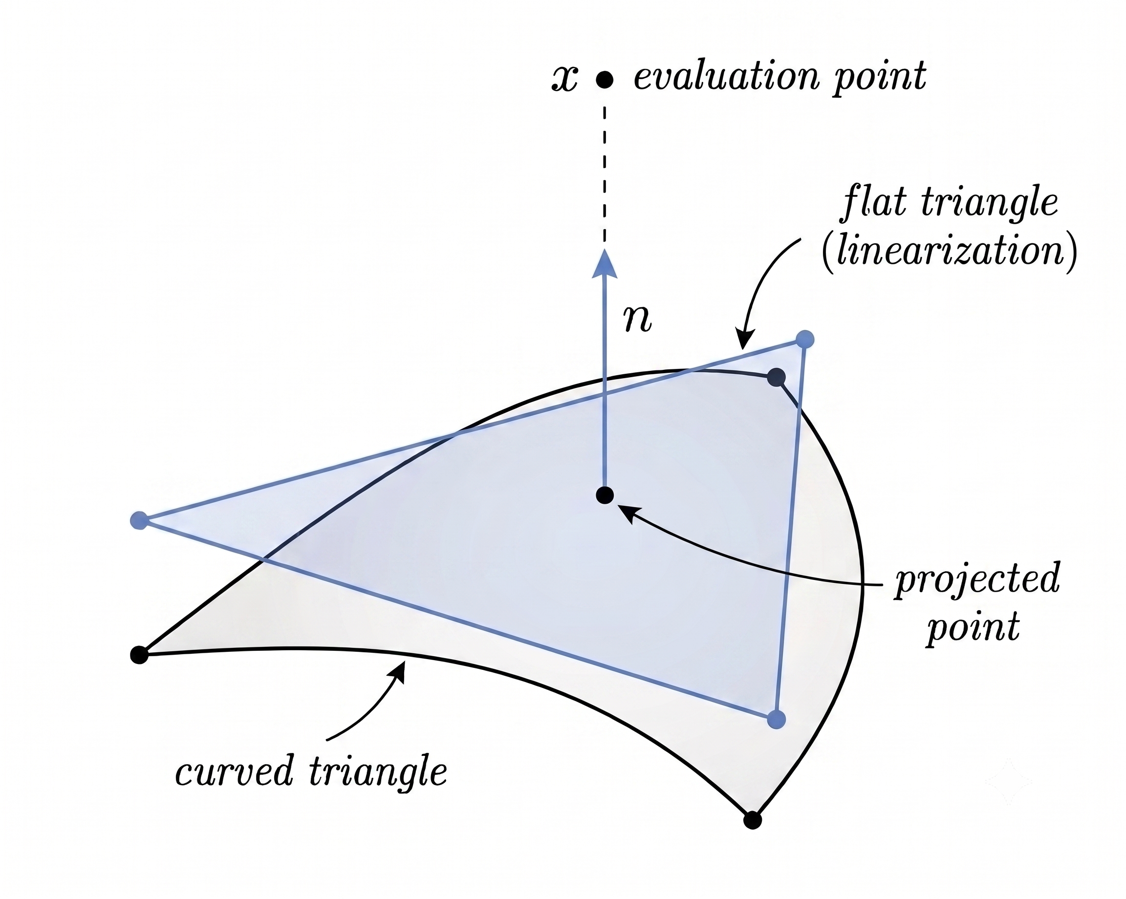
Analytical Correction

The singular correction is computed on \(\phi_{\mathrm{lin}}(\widehat T)\). Pulling the element integral back to the reference triangle gives

\[\begin{split} \begin{aligned} u_T(x) &=\int_{\phi(\widehat T)}G(x,y)\,\rho(y)\,dy\\ &=\int_{\widehat T}G(x,\phi(\widehat y))\,\widehat\rho(\widehat y)\,J(\widehat y)\,d\widehat y. \end{aligned} \end{split}\]

We add and subtract the tangent triangle:

\[\begin{split} \begin{aligned} u_T(x) &=\int_{\widehat T}G(x,\phi_{\mathrm{lin}}(\widehat y))\, \widehat\rho(\widehat x_0)\,J(\widehat x_0)\,d\widehat y\\ &\quad+\int_{\widehat T}\Big( G(x,\phi(\widehat y))\,\widehat\rho(\widehat y)\,J(\widehat y) -G(x,\phi_{\mathrm{lin}}(\widehat y))\, \widehat\rho(\widehat x_0)\,J(\widehat x_0) \Big)d\widehat y. \end{aligned} \end{split}\]

The tangent triangle captures the leading local singularity. For the Laplace kernel \(G_0(x,y)=\frac{1}{4\pi|x-y|}\) this cancels the leading \(\frac{1}{r}\) behavior, leaving a bounded remainder for standard quadrature. For Helmholtz,

\[ G_k(x,y)=\frac{e^{ik|x-y|}}{4\pi|x-y|} =\frac{1}{4\pi r}+\frac{ik}{4\pi}+O(r), \qquad r=|x-y|, \]

so the same subtraction removes the singular part and only a smooth Helmholtz correction remains. The first integral is evaluated by the exact triangle formula [GD21], the second part is evaluated using standard Gauss quadrature.

Near and Far Split

For each target point, the surface mesh is split into far elements and near elements,

\[ \mathcal T=\mathcal F(x)\,\dot\cup\,\mathcal N(x). \]

The potential is written as

\[ u(x)= \sum_{T\in\mathcal F(x)}\int_T G(x,y)\rho(y)\,dy + \sum_{T\in\mathcal N(x)}\int_T G(x,y)\rho(y)\,dy. \]

The far element integrals are smooth for this target and are evaluated using FMM. The near element integrals use the analytical correction above.