Poisson Equation BEM

We solve a Poisson problem with homogeneous Dirichlet data,

\[ -\Delta u=f \quad \text{in } \Omega, \qquad u=0 \quad \text{on } \Gamma. \]

The solution is given by the sum of a Newton potential and a single layer potential as

\[ u(x)=Nf(x)+V\rho(x) = \int_\Omega G(x,y)f(y)\,dy + \int_\Gamma G(x,y)\rho(y)\,dy, \qquad G(x,y)=\frac{1}{4\pi |x-y|}. \]

The density is determined by applying the trace operator to the representation formula

\[ V\rho=-\gamma_0 Nf \quad \text{on } \Gamma. \]

from ngsolve import *
from ngsolve.bem import *
from ngsolve.webgui import Draw
from ngsolve.krylovspace import CG

mesh = Mesh(unit_cube.GenerateMesh(maxh=0.2))
source = 32*(y*(1-y)+x*(1-x))

Volume Potential

fesL2 = SurfaceL2(mesh, order=2, dual_mapping=False)
u, v = fesL2.TnT()

fesH1 = H1(mesh, order=3)
gfs = GridFunction(fesH1)
gfs.Set(source)
with TaskManager():
    N = LaplaceSL(u*dx)(gfs)

Boundary Correction

with TaskManager():
    dsi = ds(bonus_intorder=6)
    V = LaplaceSL(u*dsi)*v*dsi
    rhs = LinearForm(-N*v.Trace()*dsi).Assemble()

rho = GridFunction(fesL2)

with TaskManager():
    pre = BilinearForm(u*v*ds, diagonal=True).Assemble().mat.Inverse()
    CG(mat=V.mat, pre=pre, rhs=rhs.vec, sol=rho.vec, tol=1e-8, maxsteps=200, printrates=False)

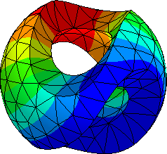
Draw(rho);

Evaluate Solution

with TaskManager():
    sol = LaplaceSL(u*dsi)(rho) + N
    Draw(sol, mesh, clipping={"vec":[0,0,-1], "function": True})